Big Data on AWS Deep Dive (Part 1): Data Lakes, Warehouses, and the Lakehouse Revolution

No code in this chapter — just mental models. Once you internalize these concepts, every AWS service you encounter later will snap into its proper place in the big data universe.

---

Why “Big Data” Exists in the First Place

Think back to the earliest backend code you ever wrote: a MySQL users table plus an orders table, and the business hummed along beautifully.

Then one day, your product manager says:

“I need the daily active users for the last 30 days, broken down by city and device model, excluding users acquired through marketing campaigns — by tomorrow.”

You write the SQL:

SELECT dt, city, model, COUNT(DISTINCT user_id)
FROM   user_activity_log              -- this table already has 5 billion rows
WHERE  dt BETWEEN '2026-04-10' AND '2026-05-10'
  AND  user_id NOT IN (SELECT user_id FROM marketing_users)
GROUP BY dt, city, model;

You submit it. MySQL grinds for 4 hours, pegs the primary database CPU at 100%, and the business team receives a flood of “order failed” customer complaints.

This is exactly the problem “big data” was created to solve:

1. Data volumes too large for a single database (hundreds of millions of rows to tens of petabytes)
2. Analytical queries and business transactions must run separately — otherwise they compete for resources and degrade each other
3. Data formats are heterogeneous: MySQL rows, Elasticsearch full-text indexes, DocumentDB documents, JSON event logs… you need somewhere to bring them all together
4. Machine learning needs access: ML engineers need to scan tens of millions of rows for a training sample — SQL is too slow, they need Parquet files that Spark can read directly

Every technology in the big data ecosystem — data lakes, Parquet, Iceberg, Spark, Flink, Athena, Glue, SageMaker — is answering one or more of these four challenges.

---

OLTP vs. OLAP: Two Database Philosophies

This is the first conceptual split you need to internalize.

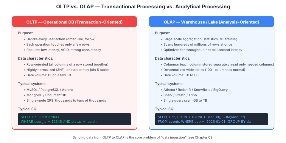
OLTP (Online Transaction Processing)

Transaction-oriented. Each operation touches only a few rows, but demands extreme speed, strong consistency, and full ACID guarantees.

• You open a food delivery app and place an order: one INSERT for the order, one UPDATE to decrement inventory, one UPDATE to deduct your balance — three SQL statements completed within 100ms
• User tables, follower tables, like tables — all OLTP workloads
• Representatives: MySQL, PostgreSQL, Aurora, MongoDB, DocumentDB

Characteristics:

• Row-oriented storage: all columns of a row are stored contiguously (reading an entire row is fast)
• Normalized schemas: avoid redundancy; multi-table JOINs are the norm
• Indexes: B+Tree supports point lookups
• Data volume: typically GB to low TB per database

OLAP (Online Analytical Processing)

Analysis-oriented. Scans billions of rows for aggregations; millisecond latency is not required — throughput is what matters.

• “What was the GMV per city per day for the past 30 days?” — that kind of query
• Representatives: Athena, Redshift, Snowflake, BigQuery, Spark SQL

Characteristics:

• Columnar storage: each column is stored independently (computing SUM(amount) only reads the amount column, not the other 99 columns)
• Denormalized schemas: wide tables with 100+ columns are normal; JOINs are avoided
• Data volume: TB to EB

Why You Cannot Use One Database for Both

It is not that it is impossible — it is that the two workloads have fundamentally incompatible performance profiles:

	OLTP	OLAP
Rows per operation	1-10	Tens of millions to billions
Expected latency	Milliseconds	Seconds to minutes
Write frequency	High (every user action)	Low (batch imports)
Consistency	Strong consistency	Eventual consistency is fine
Optimal physical storage	Row-oriented	Columnar

If you force analytical queries onto MySQL, analytics will be slow and transactions will be degraded. So modern architectures always separate them:

OLTP (business DB)  ──sync──▶  OLAP (data warehouse / data lake)
   MySQL                         S3 + Iceberg + Athena

“How do you move data from OLTP to OLAP?” — that is exactly what CDC / DMS / Zero-ETL does (see section 1.5 below and Chapter 03).

---

Data Warehouse, Data Lake, Lakehouse: Three Generations of Architecture

This is the main evolutionary arc of big data architecture. Each generation solves the previous generation’s pain points.

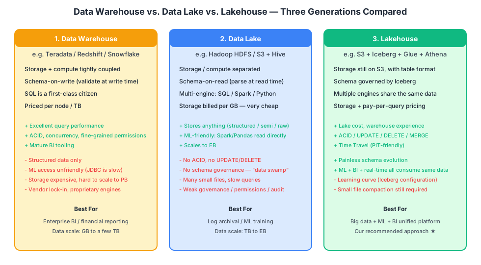
First Generation: The Data Warehouse (1990s)

Representatives: Teradata, IBM DB2 Warehouse, and later Redshift / Snowflake.

Approach:

• Dedicated hardware (early MPP — Massively Parallel Processing)
• Storage and compute are tightly coupled
• Schema must be defined before writing (schema-on-write)
• Primarily serves BI dashboards and reports

Strengths: Fast queries, full SQL support, ACID transactions. Weaknesses:

• Can only store structured data (JSON, video, and logs cannot be ingested)
• ML access is limited to JDBC — pulling data out is slow
• Storage and compute scale together — adding storage means adding compute nodes (expensive)
• Vendor lock-in

Second Generation: The Data Lake (2010s)

Representatives: Hadoop HDFS, S3 + Hive.

Core revolution:

• Storage-compute separation: S3 / HDFS only stores; Spark / Hive computes
• Schema-on-read: write whatever you want (JSON / CSV / Parquet), parse it when you read
• Low-cost storage: S3 costs pennies per GB

Strengths:

• Stores any format
• ML-friendly: Spark / Pandas read Parquet directly
• Handles EB-scale data
• Multiple engines can read the same data

Weaknesses: the “Data Swamp” problem —

• No ACID; cannot UPDATE or DELETE individual rows
• Schema chaos — nobody knows how many columns a table has
• Accidentally generates millions of small files, making queries unbearably slow
• Weak governance, auditing, and access control

Third Generation: The Lakehouse (2020s onward)

Representatives: Databricks Delta Lake, Apache Iceberg, Apache Hudi.

Core idea: Add a table format layer on top of data lake files, giving S3 directories the capabilities of a database.

Data Lake Pain Point	How the Lakehouse Solves It
Cannot UPDATE/DELETE	Iceberg maintains metadata tracking “which files are still valid”; an UPDATE actually writes new files and marks old files as obsolete
No ACID	Iceberg uses optimistic locking + metadata snapshots to implement ACID
Cannot view history	Each write creates a snapshot; Time Travel lets you go back to any historical version
Schema chaos	Iceberg enforces schemas; Schema Evolution is controlled and explicit
Small files	Compaction tasks periodically merge small files

The result: The cost of a lake + the experience of a warehouse + ML-friendliness — you get all three.

The reference architecture follows the Lakehouse pattern: S3 (storage) + Iceberg (table format) + Glue Catalog (metadata) + Athena/EMR/SageMaker (multiple engines).

---

Batch Processing vs. Stream Processing

The second mental model to distinguish: is data accumulated into batches and processed together, or processed record-by-record as it arrives?

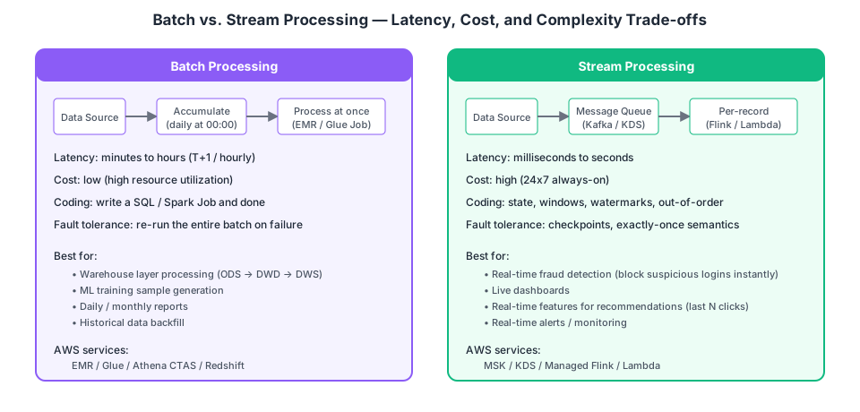
Batch Processing

Characteristics:

• Data is first accumulated somewhere (S3 / database)
• Triggered on a schedule (daily at midnight / every hour on the hour)
• Processes a large batch at once

Examples:

• Running yesterday’s GMV report at 2 AM
• Retraining a recommendation model once per day
• Data warehouse layer transformations: ODS to DWD to DWS to ADS

Typical tools: EMR Spark, AWS Glue, Athena CTAS, Redshift.

Stream Processing

Characteristics:

• Data is processed as soon as it arrives
• Runs 24/7
• State management, windowing, out-of-order events, and watermarks are everyday concerns

Examples:

• Real-time fraud detection (block a suspicious login immediately)
• Real-time dashboards (Singles’ Day GMV rolling counter)
• Real-time features for recommendation systems (last 5 clicks)
• Real-time alerting

Typical tools: Flink, Kafka Streams, Spark Streaming, Lambda + Kinesis Data Streams.

How to Choose

Business Requirement	Choice
T+1 reports, model training	Batch
Minute-level latency is acceptable	Batch (hourly / micro-batch)
Second-level latency, with recomputation needs	Stream
Always need “the current latest value”	Stream

Critical principle: prefer batch over stream whenever possible. Stream processing is an order of magnitude harder to operate, recover from failures, and maintain consistency. Start with batch, prove it works, then consider stream — this is a simple but important engineering heuristic.

In our reference architecture, the customer’s latency requirement is T+1, so the offline pipeline is primarily batch. Only future real-time feature pipelines would require stream processing (Flink).

---

CDC: Moving OLTP Data into the Data Lake

Now that we have covered the three architectural generations and batch vs. stream, let us address the most practical question: how does MySQL data get into S3?

The intuitive answer: “Write a cron job that runs SELECT * WHERE updated_at > 'last_time' every 5 minutes to export changes.”

That intuition is wrong. The following diagram explains why:

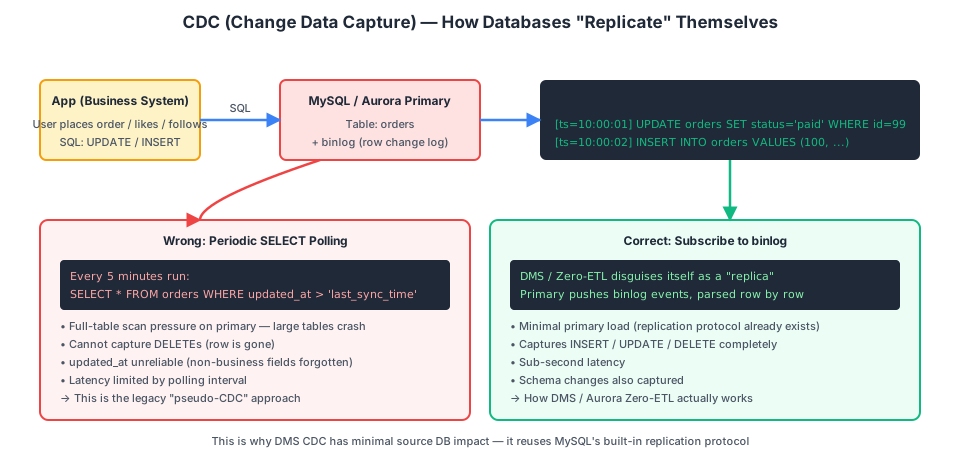
The Wrong Approach: Periodic SELECT Polling

-- Run every 5 minutes
SELECT * FROM orders WHERE updated_at > '2026-05-10 14:00:00';

Problems:

1. Puts load on the primary database: Full table scans peg the primary CPU at 100%, degrading production traffic
2. Cannot capture DELETEs: Once a row is deleted, its updated_at disappears with it
3. Depends on application-maintained fields: Is updated_at actually modified on every update? Does the application maintain it correctly?
4. Latency is bounded by polling interval: To achieve second-level latency, you would need to query every second — essentially DDoSing yourself

The Right Approach: CDC (Change Data Capture)

The core idea of CDC: do not query the table — subscribe to the database’s replication log.

MySQL has a built-in mechanism called the binlog (binary log). It is what MySQL uses for primary-replica replication — every INSERT, UPDATE, and DELETE on the source (primary) is written to the binlog, and replicas read and replay it.

What a CDC tool actually does: It disguises itself as a MySQL replica, subscribes to the binlog, parses each event row-by-row, and forwards it downstream.

App ─SQL─▶ MySQL source ─binlog─▶ DMS (disguised as replica) ─▶ S3 / Kafka / any downstream

Advantages:

• Minimal load on the source database (it was going to replicate to real replicas anyway)
• Captures INSERT, UPDATE, and DELETE completely
• Second-level latency
• Schema changes are also captured

PostgreSQL uses logical replication slots; MongoDB / DocumentDB use change streams — the principle is the same.

On AWS, CDC is primarily implemented by DMS (Database Migration Service) and Aurora Zero-ETL. Chapter 03 covers these in detail.

---

Data Layering: ODS, DWD, DWS, ADS

Once data lands in the lake, you cannot just leave raw data sitting there waiting to be queried. You must perform layered processing, for three reasons:

1. Query performance: Raw data has redundant fields and nested structures; querying it directly is slow
2. Reusability: A metric like DAU should be computed once and consumed by 100 dashboards, not recomputed by each one
3. Data governance: Cleansing, dimension enrichment, deduplication, and metric definition alignment should happen in a unified layer

The Classic Four-Layer Model

Layer	Full Name	Purpose	Example in Practice
ODS	Operational Data Store	Raw data backup layer. One-to-one mapping with source systems, almost no transformation	ods_users: mirror of the MySQL users table
DWD	Data Warehouse Detail	Detail data layer. Cleansing + standardization + dimension JOINs	dwd_user_action: event logs joined with user profile + IP-to-geo mapping
DWS	Data Warehouse Summary	Light aggregation layer. Pre-aggregated by subject/dimension combinations	dws_user_daily: each user’s daily impressions, likes, and follows
ADS	Application Data Store	Application/mart layer. Final outputs consumed directly by downstream systems	ads_user_features: 100-dimension user feature wide table for the recommendation model

Data Flow

Source Systems             Data Lake
─────────────             ───────────────────────────────────────────────
MySQL  ─CDC──▶      ods_*  ──transform──▶  dwd_*  ──aggregate──▶  dws_*  ──serve──▶  ads_*
ES     ─OSI──▶                                                                        │
DocDB  ─CDC──▶                                                                        ▼
Events ─Firehose─▶                                                   BI dashboards / ML / online services

Every layer consists of Iceberg tables, and each is produced by SQL (Athena CTAS / Spark SQL) transforming the layer above. Orchestration is handled by MWAA (Managed Airflow) or Step Functions.

---

Offline vs. Online: Two Completely Different Worlds

The last and most commonly confused concept. The data warehouse and online serving storage are two distinct layers with entirely different responsibilities.

Dimension	Offline Layer (Data Warehouse)	Online Layer (Inference Service)
Storage	S3 + Iceberg	DynamoDB / Redis / OpenSearch
Consumers	ML training / BI	User-facing request serving
Query pattern	SQL batch scans	Key-value point lookups
Latency	Seconds to minutes	Milliseconds
QPS	Tens to hundreds	Tens of thousands to hundreds of thousands
Cost model	Pay per storage + bytes scanned	Pay per QPS + capacity

A Concrete Example

A user opens their social media feed, and the app must return personalized recommendations within 50ms. Inside that request:

1. Look up user features (age, city, recent interest tags) — cannot query the data warehouse; must do a point lookup from a KV store like DynamoDB
2. Retrieve recall candidates (1,000 items this user might be interested in) — from DynamoDB / OpenSearch
3. The ranking model scores all 1,000 candidates — SageMaker Endpoint
4. Return the Top 10

Why can you not just query the data warehouse directly?

• Athena’s startup + parsing + queueing overhead alone is hundreds of milliseconds to seconds — a 200ms budget cannot accommodate that
• Athena charges per bytes scanned; each recommendation scanning several MB at 100,000 QPS would exhaust your budget in a single day
• Athena is an OLAP analytics engine, not a high-QPS OLTP service — its architecture fundamentally does not match high-concurrency point lookups

So modern recommendation architectures always look like this:

Offline warehouse (S3 + Iceberg)       ──daily batch sync──▶      Online storage (DynamoDB + Redis)
ads_user_features                                                  user_features (KV)
ads_recall_pool                                                    recall_candidates (KV)
                                                                          │
                                                                          ▼
                                                            Recommendation service (ms-level response)

Chapter 06 will draw the complete offline pipeline for our reference architecture; Chapter 08 covers how to choose between different online storage options.

---

Chapter Summary

Concept	One-Liner
OLTP vs. OLAP	Business database vs. data warehouse — two different workloads with fundamentally different physical storage structures
Data Warehouse	Legacy generation: coupled storage and compute, structured data only, ML-unfriendly
Data Lake	Storage-compute separation, stores anything, but no ACID — easily becomes a swamp
Lakehouse	Data lake + table format (Iceberg) — best of both worlds
Batch vs. Stream	Accumulate and process together vs. process one-by-one as it arrives; prefer batch when possible
CDC	Subscribe to database binlog for real-time sync — never poll
Data Layering	ODS to DWD to DWS to ADS, each layer an Iceberg table
Offline vs. Online	Data warehouse is not online storage; a 50ms recommendation response cannot query Athena