What is the recommendation system funnel?

The funnel narrows candidates in stages: Recall (10M→1K items via multiple channels), Pre-Ranking (1K→100 via lightweight model), Ranking (100→50 via deep model like DeepFM), and Re-Ranking (50→10 with diversity rules). Total P99 < 200ms.

What is Point-in-Time (PIT) correctness in ML training?

PIT means using feature values as they existed when the event occurred, not current values. Without PIT, you get feature leakage — the model trains on 'future' data that won't be available at inference time, leading to poor online performance.

Big Data on AWS Deep Dive (Part 7): Recommendation System Fundamentals — Funnel, Two-Tower, and PIT

Q: What is Point-in-Time (PIT) correctness in ML training?

PIT means using feature values as they existed when the event occurred, not current values. Without PIT, you get feature leakage — the model trains on 'future' data that won't be available at inference time, leading to poor online performance.

Once data lands in the lake, the ultimate goal is to serve recommendation algorithms. This chapter covers recommendation systems from scratch: the recall-ranking funnel, feature engineering, model types, and why PIT correctness is the critical lifeline.

No ML background assumed — just familiarity with code and basic concepts like “vector” and “dot product.”

What Problem Does a Recommendation System Solve?

When you scroll through TikTok, Instagram, or YouTube, you see different content every time you open the app — there is a recommendation system working behind the scenes.

It must answer: “From hundreds of millions of candidates, which 10 items should this specific user see? Decide within 200ms.”

The challenges:

Too many candidates: Platforms receive tens of millions of new uploads daily with hundreds of millions of active users
Strict latency: User-perceived response must be under 200ms
Personalization at scale: Every user has different preferences
Real-time feedback: If a user taps “not interested,” the next refresh must reflect that
Cold start: New users have no history; new content has no engagement data

Scoring and ranking every candidate for every user is computationally impossible within latency budgets. That is why we need a multi-stage filtering “funnel.”

The Recommendation Funnel: 4–5 Stages

Recsys Funnel

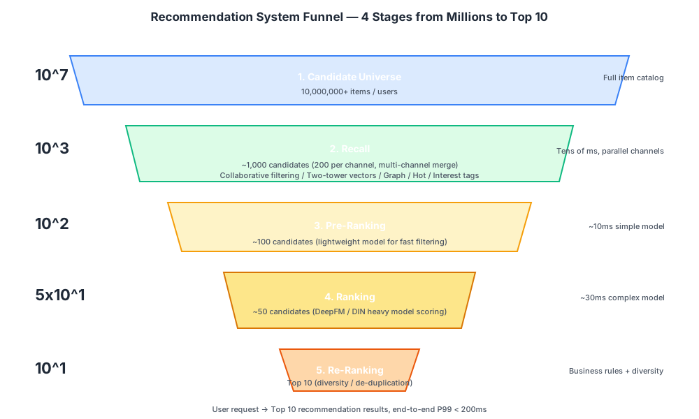
Stage 1: Candidate Pool (10^7 scale)

The entire content library or user graph. This is the raw source data.

Stage 2: Recall (down to 10^3)

Quickly filter hundreds of millions of candidates down to a few hundred or thousand for downstream models to score.

Multi-channel recall — run N different retrieval methods in parallel, then merge results:

Recall Channel	Method	Data Source
Collaborative Filtering (U2U-CF / I2I-CF)	“Users similar to you liked these”	Historical interaction matrix
Two-Tower vector recall	User vector → find nearest-neighbor item vectors	Model training + vector store
Graph recall (GNN)	Propagation over social graph	Neptune + Neptune ML
Popularity recall	Global / regional trending	Real-time statistics
Interest tag recall	Tag matching	Tag inverted index
Contextual recall	Same city / followed friends’ content	Business rules

Each channel retrieves 200–500 items; after deduplication, roughly 1,000 candidates remain. This step runs in single-digit milliseconds thanks to precomputation and indexing.

Stage 3: Pre-Ranking (down to 10^2)

Pre-ranking is the intermediate filtering layer between recall and fine ranking (another 10x reduction). It uses a lightweight model for fast scoring (e.g., Logistic Regression, shallow MLP) to stay within latency budget.

Stage 4: Ranking (down to 10^1)

Heavy models (DeepFM / DIN / DCN-V2, etc.) meticulously score the remaining few dozen candidates. This stage is the main battlefield for model innovation — nearly all optimization efforts focus here.

Stage 5: Re-Ranking

Business rules + diversity constraints:

Spread out same-category content
Filter already-viewed items
Mix in ads / followed friends’ content
Exposure protection for cold-start new content

The final Top 10 is sent to the frontend.

Recall vs. Ranking: The Fundamental Difference

Many people conflate these two stages. Here are the key differences:

	Recall	Ranking
Goal	Don’t miss (recall)	Rank accurately (precision)
Candidate scale	Hundreds of millions → thousands	Thousands → tens
Model complexity	Lightweight (two-tower separation + ANN)	Heavy (DeepFM / Transformer)
Online latency	Tens of ms	Tens of ms
Features	More global-level features	More fine-grained cross features
Training cost	Medium	High

Two-Tower Recall Model in Detail

The most classic and widely-used recall model in social scenarios.

Two Tower

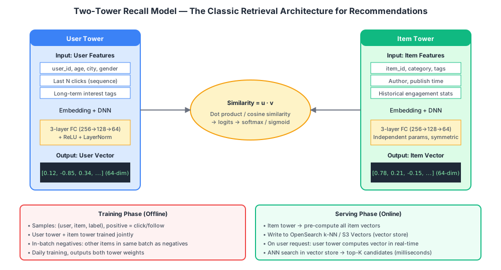
Model Architecture

Two independent neural networks (“towers”):

User tower: Consumes user features → outputs a 64-dim or 128-dim vector
Item tower: Consumes item features → outputs a vector of the same dimensionality
The dot product or cosine similarity of the two = the user’s preference score for the item

score(user, item) = user_embedding · item_embedding

Training

Samples = (user, item, label), where positive samples are actual clicks or follows.

Key technique — in-batch negatives: Other users’ positive samples within the same batch serve as negative samples for the current user (no need to explicitly sample negatives).

Loss functions: softmax cross-entropy / sampled softmax / BPR loss.

Serving (The Key Insight)

Why the two-tower model is easy to deploy — because the user tower and item tower are decoupled, enabling offline precomputation:

After training:
  1. Use the item tower to precompute vectors for every item on the platform
     (tens of millions of items × 64 dimensions)
  2. Write all vectors into a vector store (OpenSearch k-NN / S3 Vectors)
  3. When a user request arrives, only run the user tower in real-time
     to compute the user vector (< 10ms)
  4. Query the vector store for the K nearest neighbors (millisecond-level ANN search)
  5. Return top-K candidate items

→ This is the essence of how two-tower enables "real-time recall":
  item vectors precomputed + ANN retrieval

ANN: Approximate Nearest Neighbor

With hundreds of millions of item vectors, exact nearest-neighbor search is too expensive. So we use approximate algorithms:

HNSW (Hierarchical Navigable Small World) — current mainstream
IVF + PQ — Faiss family, quantization saves memory
ScaNN (Google)

Sacrificing minimal precision (recall@100 drops 1–2%), latency goes from seconds to milliseconds.

OpenSearch k-NN supports Faiss / Lucene / nmslib backends: as of 2026, Faiss is the production choice (best performance + quantization + GPU support). Lucene suits small-scale pure-JVM use cases. nmslib is deprecated and should no longer be used.

Feature Engineering: 90% of the Work Lives Here

“Garbage in, garbage out.” — Feature quality determines the model’s upper bound.

Feature Categories

User-side:

Static: age, gender, city, registration age
Short-term behavior: last 5 clicks, dwell time in the past hour (real-time features)
Long-term preferences: frequently viewed tags, time-of-day patterns, traffic sources
Social: follower count, following count, friend activity level

Item-side:

Static: author, category, tags, creation time
Statistics: impressions, CTR, like rate, completion rate
Dynamic: trending status, recent comment count

User-Item cross features:

User’s historical interactions with this author
User’s preference score for this tag
Similar content the user recently viewed

Context:

Time (morning / afternoon / evening), day of week, holidays
Device, network (WiFi / cellular)
Geographic location

How Features Are Organized in the Data Warehouse

ads_user_features        -- User-side (daily batch update)
  user_id, age, city, last_5_click_tags, ...

ads_post_features        -- Item-side (hourly update)
  post_id, category, ctr_7d, like_rate, ...

ads_user_pair_features   -- Cross features (on demand)
  user_id, target_user_id, common_tags, ...

user_realtime_features   -- Real-time (DynamoDB / Flink maintained)
  user_id, last_click_seq[5], session_duration, ...

Feature Data Flow

[ods_event] → [dwd_user_action] → [dws_user_daily] → [ads_user_features]  ← daily batch
                                                          │
                                                          ▼
                                                  Sync to DynamoDB
                                                          │
                                                          ▼
                                                  Real-time point lookup at inference

[MSK events] → Flink real-time compute last 5 clicks → DynamoDB user_realtime_features
                                                          │
                                                          ▼
                                                  Real-time point lookup at inference

PIT Correctness (The Most Common Pitfall)

PIT

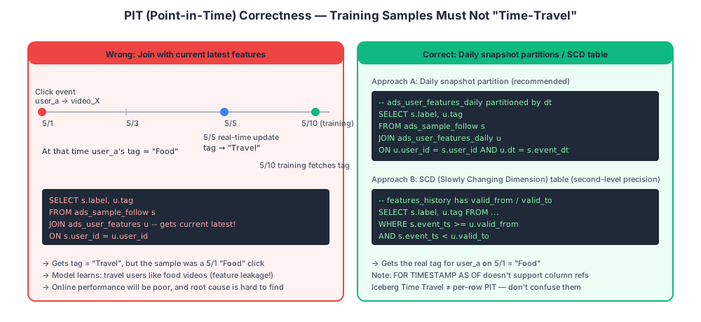
The Problem

Training samples must use feature values as they existed at the moment the event occurred, not the latest current values.

Otherwise → feature leakage: the model uses “future” information, offline AUC looks great, but online performance is terrible.

Example

On May 1, User A clicks Video X (a positive sample)
On May 1, A’s interest tag = “food”
On May 5, A browses videos and the algorithm updates the tag to “travel”
On May 10, during training, a naive JOIN ads_user_features ON user_id = A → retrieves “travel”
The model learns: “travel” users click food videos → wrong

Solutions

Warning: Correcting a widespread misconception: Many articles suggest JOIN ads_user_features FOR TIMESTAMP AS OF s.event_ts — this is incorrect. In Iceberg / SQL:2011, FOR TIMESTAMP AS OF only accepts literal constants, not column references. See Ch02 Section 2.5 on PIT for details.

Solution A: Daily Feature Snapshot Partitions (Recommended, Most Common)

-- ads_user_features_daily partitioned by dt, with a full snapshot written daily
SELECT s.label, u.tag, u.age
FROM   ads_sample_follow s
JOIN   ads_user_features_daily u
       ON u.user_id = s.user_id
       AND u.dt    = s.event_dt;   -- Join on the day's snapshot

Precision: day-level. Use Iceberg expire_snapshots to control storage costs.

Solution B: Slowly Changing Dimension (SCD Type 2, second-level precision)

user_id  tag    valid_from           valid_to
A        food   2026-04-01 00:00     2026-05-05 12:00
A        travel 2026-05-05 12:00     2999-12-31 23:59

SELECT s.label, u.tag
FROM   ads_sample_follow s
JOIN   ads_user_features_history u
       ON s.user_id = u.user_id
       AND s.event_ts >= u.valid_from
       AND s.event_ts <  u.valid_to;

Precision: second-level. More storage-efficient (only adds rows on changes).

Solution C: SageMaker Feature Store

A managed PIT feature store; call get_record(record_id, event_time) and it automatically returns the value as of that moment. Under the hood, it wraps Solution A/B. See Ch09 for details.

Iceberg Time Travel: Real Value Beyond PIT

Although it cannot do per-row PIT joins, Time Travel remains critical for:

Data rollback: Recover from accidental deletes or updates
Reproducible training: Pin a snapshot ID to produce identical samples months later
Auditing / debugging: Compare “yesterday’s table at midnight” with “today’s table at midnight”

→ The complete solution for recommendation scenarios is Iceberg + daily snapshot partitions + SCD tables. Time Travel is an auxiliary capability.

Why This Is the Critical Lifeline

New ML engineers building training samples almost always make this mistake. Offline AUC of 0.85 looks beautiful, but online CTR doesn’t budge — the root cause is feature leakage. This is the “classic pitfall” of recommendation engineering. Choose from Solution A/B/C — do not go down the non-existent path of per-row Time Travel.

Real-Time Features: What Flink Does

Some features are short-lived and high-frequency, requiring real-time maintenance:

Real-Time Feature	Description
Last 5 clicks	Behavior sequence for DIN-style models
Dwell time in the last hour	Interest intensity signal
Current session action sequence	Short-term intent modeling
Current network / device / time slot	Context

Implementation:

MSK events
   │
   ▼
Flink Job (keyBy user_id)
   │
   ├─ Sliding Window (5 min)
   ├─ State: maintain each user's last N clicks list (RocksDB)
   │
   ▼
DynamoDB user_realtime_features
   user_id → { last_5_clicks: [...], session_dur: 300, ... }
   │
   ▼
Recommendation inference service point lookup (milliseconds)

Latency: from user click → visible in DynamoDB, single-digit seconds.

Model Type Overview

Recall Models

Model	Use Case
Collaborative Filtering (CF)	Classic; works as long as you have an interaction matrix
Two-Tower	Mainstream; essential for social scenarios
Graph Neural Network (GNN)	Effective when relationship data is rich (social networks)
Sequential Models (SASRec / BERT4Rec)	Behavior sequence modeling

Ranking Models

Model	Use Case
LightGBM / XGBoost	Simple and reliable; strong feature engineering can beat many deep models
DeepFM	DNN + FM; balances feature crossing and depth
Wide & Deep	Google’s classic architecture
DIN (Deep Interest Network)	Alibaba; attention over behavior sequences
Transformer	Heavy; excellent results but expensive
MMoE / PLE	Multi-task (optimize click + completion + follow simultaneously)

Practical Recommendations for Customer Scenarios

POC phase (within 6 months):

Recall: Collaborative Filtering + Two-Tower (OpenSearch k-NN)
Pre-ranking: Can be omitted
Ranking: LightGBM (first) → DeepFM
Re-ranking: Business rules (diversity, spread)

Advanced phase:

GNN recall (Neptune ML)
DIN / SIM ranking (behavior sequence modeling)
Multi-channel recall fusion (learned weights)

Offline Evaluation Metrics

Metric	Stage	Meaning
Recall@K	Recall	Does top-K retrieval hit the actual clicks?
Hit Rate	Recall	Similar to Recall
AUC	Ranking	Discrimination ability (0.5 = random, 1.0 = perfect)
NDCG@K	Ranking	Weighted ranking quality
GAUC	Ranking	AUC computed per-user then weighted (closer to online performance)

Warning: High offline AUC does not equal good online performance. Common causes: PIT errors, data leakage, ignoring exposure bias. A/B testing is the ground truth.

A/B Testing

Deploying a model does not mean rolling it out to all users immediately. You must A/B test:

All users
  ├─ 50% (Control group A) → Old model
  └─ 50% (Experiment group B) → New model

Observe for N days, compare core business metrics:
  - CTR (Click-Through Rate)
  - User dwell time
  - Retention rate
  - GMV / Business conversion

If the new model is significantly better (statistically p < 0.05 and business metrics improve) → full rollout.

A/B testing platforms are often built in-house (GrowthBook / Optimizely / custom); this guide does not expand on that topic.

Chapter Summary

Concept	One-Liner
Recommendation Funnel	Candidate pool → Recall → Pre-Rank → Rank → Re-Rank
Recall	Don’t miss; hundreds of millions → thousands; multi-channel parallel
Ranking	Rank accurately; thousands → tens; heavy models
Two-Tower	Mainstream recall model; item tower precomputed + ANN retrieval
Feature Engineering	User / item / cross / context; 90% of the work
PIT	Use feature values from the moment of the event; leverage Iceberg Time Travel
Real-Time Features	Flink maintains short-term high-frequency features; writes to DynamoDB